Using a Bayesian Inference (BI) approach

Bayesian Inference (Rannala and Yang, 1996; Yang and Rannala, 1997) randomly estimates the model parameters across a statistical distribution resulting in different trees. The likelihood of the trees are computed a posteriori (actually they are approximated by Markov Chain Monte Carlo -MCMC- methods) resulting in posterior probabilities, which can be understood as the probability of a tree being right given the randomly selected model parameters.

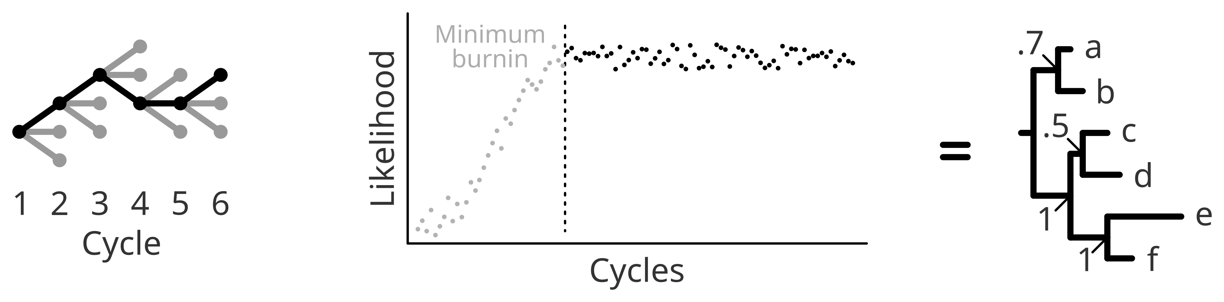
Briefly, bayesian Inference collects information along the way to update and improve the model parameters. A single inference will most likely yield a rather poor tree, since the search for model parameters is predefined or random (to an extent). Yet in the following cycles (sometimes also called iterations, generations or even chains) model parameters are going to be adjusted based on previously collected information resulting in trees with higher and higher likelihood. In this sense, the number of generations will affect the random sampling, and therefore your results.
It is recommended to monitor the likelihood per cycle to be sure that your model optimization is arriving to a convergence. Normally, a safe option is to opt for a very long chain, but an excessively long chain might result in a waste of computational resources. If you are interested in a trade-off between ensuring convergence and not spending several days, weeks or months in a redundant analysis you can, for example, explore the Effective Sample Size of the MCMC run in the software Tracer.
Because of the long sampling, when you choose a Bayesian approach it is very important to check the likelihood over the different cycles and remove the “learning slope”, normally referred to as burn-in.

Bayesian approaches are available in many different softwares. Such as MrBayes, BEAST, BEAST2 or PhyloBayes. Yet, they need most of the times to be run in different blocks, where different parameters need to be set that will influence your analysis. Instead of running them from a single command, as we did for ML approaches, here we save all our options in a simple text (or xml) file and we run the file within the BI software.

Here you have an example of a script to be run using MrBayes, let’s save it as “phylo_mrBayes.nexus”:

begin mrbayes;
	set autoclose=yes nowarn=yes;
	execute FILE.nexus;
	lset nst=6 rates=gamma;
	mcmc ngen=10000000 Nruns=4 savebrlens=yes file=OUTPUT;
	sump;
	sumt;
end;

#The mcmc command assumes a burnin of 25%: relburnin=yes and burninfrac=0.25

That can be run as follows:

mb phylo_mrBayes.nexus > ${OUTPUT}_mrBayesgamma.log

Something to bear in mind is that MrBayes uses “nexus” format and not “fasta”. This can be easily exported/transformed in AliView.

Alternatively, you can type each one of the lines from the script that we called phylo_mrBayes.sh directly in the MrBayes prompt (except for the first line, which sets the auto closing).

And in this script (phylo_BEAST.xml) you can find an example of a BEAST xml file in its most simple format (don’t panic! such xml file can be created through the graphical user interface package BEAUti), that can be run as follows:

beast -seed $RANDOM -beagle_SSE phylo_BEAST.xml

And now we have to summarise the chain with treeannotator:

treeannotator -burnin 1000000 -heights median OUTPUT.trees OUTPUT_mcmc.tre

The main problem (or advantage, depends on your question) is that BEAST assumes a clock model. But the molecular clock concept is getting out of scope. If you are very interested, please have a look at this excellent practical guide to molecular dating published by Hervé Sauquet (2013), and if you already have a solid tree that you want to date in time, you can have a look at MCMCTree from the PAML package.